Wednesday 29 July 2015

IBM Cognos Proven Practices: IBM Cognos BI – Working with Multiple Relational Data Sources

Introduction

Purpose

This document will provide guidelines around working with multiple relational data sources in Framework Manager and recommendations on how to improve performance in various scenarios.

Applicability

This document was written and tested against IBM Cognos 8.4.1 and IBM Cognos 10.1.

Exclusions and Exceptions

This document does not cover working with multiple OLAP sources.

Assumptions

This document assumes readers have experience with IBM Cognos BI, in particular IBM Cognos Report Studio and IBM Cognos Framework Manager.

Overview

Many organizations are faced with disparate data sources and the task of trying to consolidate this information for reporting and analysis. Although you may want to consolidate all your data into a single relational database for reporting purposes, it may not be feasible, financially viable, or may take quite some time to implement and require an interim BI solution.
IBM Cognos BI provides facilities to bring these disparate data sources together for reporting purposes, but there are several considerations that should be taken into account before embarking on a BI project.
This document will look at the different ways of dealing with disparate data sources and identify the pros and cons to each method. It will also provide tips on how to reduce performance impact where applicable.

Data Access Strategies

Before beginning data access to your company's data for reporting purposes, you may want to ask some of the following questions with regard to the data and how it will be consumed.
  • How fresh does the data need to be? Are you reporting on yearly, quarterly, monthly, weekly, daily, hourly, or even up to the second data? Knowing this information can help you decide how to access or store your reporting data. Is a data mart or warehouse the way to go, can a cube be used, or must you go against live data?
  • Will users of the data mainly look at summarized data or require an interactive experience (drill up and down through the data)? If so, then perhaps an OLAP package or dimensionally modeled relational (DMR) package should be considered. See DMR note below for more information.
  • Is the data available able to support your business questions? For example, lack of conformed product data throughout the company can prevent querying product metrics across the divisions in the company. Product data in one division should mean and be represented the same way in all divisions. This way metrics from all divisions can be compared through the conformed product data.
These questions are just some examples of the challenges you may be faced with when trying to implement a BI project. Although OLAP technology has been mentioned, this document will focus on accessing multiple relational data sources only.
Note: Dimensionally modeled relational (DMR) modelling is a capability that IBM Cognos Framework Manager provides allowing you to specify dimensional information for relational metadata. This allows for OLAP-style queries. Where possible, using OLAP technologies will typically provide better performance, but DMR may sometimes be appropriate where smaller data sets are concerned (one less technology to implement in the project) or if OLAP-style queries are required on live data.

Do you Really Need to Create Joins Between Databases?

One of the first questions you will want to ask when dealing with disparate data sources is, “do I actually need to join these data sources together?” Do you simply require displaying the data in the same dashboard or report, but without a physical join? Each database can have it's own query in a dashboard or dashboard-style report and be displayed along side each other without a physical joining of the data. In other words, co-locate the data. For example, executives may want to see the weekly correlation between weather statistics and outdoor product sales. Each is contained in a different database. A join between these two databases may not be necessary if they just want to see what the weather was on a given day of sales and quickly see a visual trend of increased sales on warmer days. Each of these queries can be represented in a list or graph and displayed side-by-side in a dashboard or dashboard-style report.
In these types of scenarios, performance concerns due to local join processing of data on the IBM Cognos BI servers are avoided.

Are Joins or Master/Detail Relationships Better?

There will be instances where you simply must relate the data from disparate data sources for certain reports. For example, each region of a company may manage it's own account information in one database while transactional sales figures are recorded in a central system. Each region may want to use their account data to filter the sales records.
IBM Cognos BI supports relating disparate databases in either Framework Manager or Report Studio. In the example we are using, a relationship can be created between the regional Account table from one database to the Sales table in the other database. The effect of this, however, will produce local data processing on the IBM Cognos BI servers. Each database will be queried for a potentially significant amount of data and then joined locally to filter out unwanted records. To see if performance is acceptable, you may want to apply some basic math to anticipated queries and, of course, test them in your environment. What is the amount of data in table X that you would request and then join to a certain amount of data in table Y? For smaller data volumes or cases where reports are run infrequently (perhaps scheduled once a week during off peak hours), creating cross-database joins may be a perfectly acceptable and simple solution.
For larger data sources however, this may present longer wait times for report output and may not be an optimal solution. Consider the example where the Sales table has several million rows, but each region is only interested in a few hundred thousand, the extra processing may not yield acceptable wait times. In these cases, Report Studio report authors can use master/detail relationships as an alternative. Master/detail relationships will retrieve the master data first, in this case from Accounts, and then for each account retrieve the related Sales records. This technique will generated more queries to the detail table database, but each query will be filtered.
By implementing master/detail relationships, performance can be increased by reducing the amount of records returned by the database on the detail side, however, as with any technique, there are thresholds. If the master query table has a large volume of data, perhaps millions of rows, then there might be an unacceptable amount of queries issued to the database table on the detail side.

Working with Single Instances of a Database Vendor

Understanding Differences in Relational Database Vendor Technologies

When dealing with relational databases and IBM Cognos BI, you may encounter situations where you are joining items from the same database vendor instance, but through different IBM Cognos BI data source connections defined in IBM Cognos Connection. In these scenarios, the BI servers will locally join the data from the various defined BI data source connections. This behavior may or may not be desired. If it is not desired, you can configure Framework Manager to push the processing to the database vendor.
The following will explain how different database vendor technologies behave, how metadata appears during import in Framework Manager, and finally how to configure your model so that processing is pushed to the database if desired.
There are a few different scenarios for how database vendors deal with the qualification of their objects. For example, some vendors only have the concept of instance and a collection of objects such as tables, indexes, and so on. This document will focus on two of the most typical scenarios which will be labeled Scenario A and Scenario B.
Scenario A – Instance and Schemas
In Scenario A, the vendor has the concept of instance (the database software running on a computer) and schemas (also referred to as “user” by some vendors). Illustration 1 below illustrates a single instance named A containing four schemas named A, B, C, and D. A vendor example of this scenario is Oracle.
Illustration 1: Scenario A - instance and schemas
Scenario A - instance and schemas
In IBM Cognos BI, in this scenario, you can create one IBM Cognos BI data source for the database vendor instance and have access to all schemas within it. Illustration 2 below shows the Select Objects screen of the Framework Manager Metadata Wizard import process where the instance name (Oracle) is at the top of the metadata tree and the various schemas such as CM, GOSALES, and so on, are direct children of the instance.
Illustration 2: Framework Manager Metadata Wizard showing Oracle example of instance and schemas
Framework Manager Metadata Wizard showing Oracle example of instance and schemas
You are free to import items from multiple schemas and join tables from the different schemas as required. In this scenario, IBM Cognos BI will push cross-schema join processing to the database vendor providing it supports the query.
Scenario B – Instance, Catalogs, and Schemas
In Scenario B, the vendor has the concept of instance (again, the database software running on a computer), catalogs (also referred to as “database” by some vendors), and schemas (again, also referred to as “user” by some vendors). Illustration 3 below shows a single instance named A with two catalogs named A and B. Catalog A contains two schemas named A and B, and Catalog B contains two schemas named C and D. A vendor example of this scenario is Microsoft SQL Server.
Illustration 3: Scenario B - instance, catalog, and schemas
Scenario B - instance, catalog, and schemas
In this scenario, in IBM Cognos BI, you must create one IBM Cognos BI data source per catalog you wish to import. Illustration 4 below shows the Select Objects screen of the Framework Manager Metadata Wizard import process where the instance name (GOSALES) is at the top of the metadata tree, followed by the catalog name (GOSALES), and below that the various schemas such as gosales, gosaleshr, and so on.
Illustration 4: Framework Manager Metadata Wizard showing Microsoft SQL Server example of instance, catalog, and schemas
Framework Manager Metadata Wizard showing Microsoft SQL Server example of instance, catalog, and schemas
In Scenario B, if you wish to import additional metadata from other catalogs, you will need to do so through another IBM Cognos data source connection for each catalog. Once you have the items imported from the various catalogs, you can join items from one catalog to another. For example, Illustration 5 below shows a table from the C8-Bursting catalog (database) joined to a table in the GOSALESDW catalog (database) from the same SQL Server instance.
Illustration 5: Framework Manager diagram illustrating a join between two SQL Server databases from the same instance
Framework Manager diagram illustrating a join between two SQL Server databases from the same instance
However, when you query items from the joined query subjects from each catalog, IBM Cognos BI will treat each catalog as a different data source instance since there is not enough information to indicate that it is the same instance. In fact, even if you created two data sources in IBM Cognos BI to the same instance and catalog and joined between them, IBM Cognos BI would still treat them as separate instances. In any case, this will prevent IBM Cognos BI from pushing the join between the catalogs to the database vendor. This can be seen by examining the native SQL of such a query.
For example, a query with Recipients from Burst_Table and SALES_TARGET from SLS_SALES_TARGET_FACT produces the SQL shown in Illustration 6. The Cognos SQL in this Illustration shows a join between the tables, but the native SQL does not. It shows two separate select statements (highlighted below). This indicates that two separate result sets will be retrieved and joined locally on the IBM Cognos BI servers.
Illustration 6: Framework Manager test result showing Native SQL with two separate select statements
Framework Manager test result showing Native SQL with two separate select statements
If the desired approach is to push the join to the database instance, you simply need to change the Data Source properties in the Framework Manager model to all point to one IBM Cognos BI data source connection.
In this example there are two data sources involved, each with different property settings as seen in Illustrations 7 and 8. The Content Manager Data Source property for the great_outdoors_warehouse data source points to great_outdoors_warehouse and the same property for the C8-Bursting data sources points to C8-Bursting.
Illustration 7: Framework Manager - Data Source Properties pane for great_outdoors_warehouse data source
Framework Manager Data Source Properties pane for great_outdoors_warehouse data source
Illustration 8: Framework Manager - Data Source Properties pane for C8-Bursting data source
Framework Manager Data Source Properties pane for C8-Bursting data source
To push the join between the two catalogs down to the database vendor, simply have both Content Manager Data Source properties point to the same IBM Cognos BI data source name. This tells IBM Cognos BI to use the same data source instance but different catalogs within that instance. In this example, the C8-Bursting data source will have its Content Manager Data Source property changed to point to great_outdoors_warehouse as shown in Illustration 9.
Illustration 9: Framework Manager - Data Source Properties pane with Content Manager Data Source name changed to match the great_outdoors_warehouse data source name
Framework Manager Data Source Properties pane with Content Manager Data Source name changed to match the great_outdoors_warehouse data source name
Now, when the same query is run, the native SQL that is generated is a single select statement joining the two tables from the different catalogs at the database tier as shown in Illustration 10.
Illustration 10: Framework Manager test result showing Native SQL with a single select statement after changing the Content Manager Data Source property
Framework Manager test result showing Native SQL with a single select statement after changing the Content Manager Data Source property
A single select statement is generated and the join is pushed to the database.

Working with Multiple Database Instances or Vendors

As already stated earlier in this document, you can join disparate databases in IBM Cognos Framework Manager, but by doing so, local processing of the joins between the databases will occur on the IBM Cognos BI servers. If this is not desirable, you may want to consider federation technologies.
Most major database vendors offer some form of federation technology which allows you to incorporate tables from other databases in your vendor's environment. This includes creating relationships with these tables and various forms of optimization such as hints or data caching to name a couple. This document will not go into detail about vendor specific federation technologies. You will need to refer to their documentation for specifics. The point of this section is to point out that federation technologies exist and may benefit you in terms of optimizing the disparate data sources for reporting in IBM Cognos BI.
There are also other third-party database federation tools that may also be of interest or provide additional benefits. For example, IBM offers IBM Cognos Virtual View Manager (VVM), which can be used to create a securely managed unified view across files, databases, and packaged applications. Once you are satisfied with your VVM model, it can act as an ODBC data source for IBM Cognos BI. Again, it provides optimization such as hints and data caching. VVM also provides access to streaming XML and has additional data services for Siebel, SAP, and Salesforce.com.

When to Consider Tactical ETL

There may be scenarios where most of the data you require for reporting exists in one database with the exception of a few other key tables. Rather than build a new warehouse to consolidate all the data into one database, perhaps it might make sense to simply extract transform and load (ETL) the data from the other system or systems into the main database of interest. There are several ETL tools on the market. IBM offers IBM InfoSphere DataStage or IBM Cognos Data Manager as an example.
Consider the generic example in Illustration 11 where Database 1 has two tables joined together, Table 1 and Table 2, and Database 2 has three tables joined together, Table 3, Table 4 and Table 5.
Illustration 11: Two disparate data sources
Two disparate data sources
Imagine that Database 2 has the majority of data required for reporting but requires data from Table 1 located in Database 1. You can ETL the required data from Table 1 into Database 2, as seen in Illustration 12, and join the new table as required to ensure join processing is all done in Database 2.
Illustration 12: ETL Table 1 from first data source into second data source
ETL Table 1 from first data source into second data source

Use a Star Schema Data Mart or Warehouse

Up until this point we have looked at methods of disparate database reporting other than data marts or warehouses. This is because it is not always feasible to consolidate enterprise data into a data mart or warehouse. However, if time, expense, and resources are not a road block, the ideal scenario is to work towards a star schema design for a data mart or warehouse using an ETL tool and aggregate data where possible. When your enterprise data is consolidated and structured according to the industry standard star schema design, reporting on the data is easier to accomplish and performance is usually much better. Another benefit is that once the data is in this type of structure, it is easier to extend the data into cubes for OLAP querying since most of the dimensional design (measures and related dimensions) has been done.
This document will not go into details of star schema design. The intent is to provide guidance around what methods are available to consolidate multiple data sources for BI reporting.

Working with the External Data Feature in IBM Cognos 10

In IBM Cognos 10, there is a new feature called External Data which can be leveraged in Report Studio and the new Business Insight Advanced studio. This new feature allows authors to connect to personal data sources such as Excel spreadsheets, tab or comma delimited files, or XML files that adhere to IBM Cognos XML schema, and link them to data items in an existing IBM Cognos BI package. Illustration 13 shows an external file linked to a query item in the Retailers query subject of an existing package called GO Sales (query).
Illustration 13: Linking external data to an existing package
Linking external data to an existing package
As with other disparate data source scenarios in this document, joining external data to your existing package will incur some form of local processing on the IBM Cognos BI servers. Also, as with other scenarios described in this document, you can choose to author a query that joins the two data sources or use master/detail relationships. The latter may show better performance. For joins, again, two separate queries will be generated and processed for each data source and the result sets will be joined locally. For master/detail relationships, more queries will be generated for the database on the detail side based on the results of the master query, but each one will be filtered by the master query thereby generating more efficient detail queries.
So even in the case of external data queries, it is important for authors to know the implications of their actions and make decisions that best suite their needs and performance requirements.

Advanced Sorting in Report Studio

Usually if we have data(Reinsurer Name) with Upper and Lower case mixed then Cognos will sort in a different manner

If suppose we want Reinsurer Name to be sorted in proper way and not in the way the cognos does then we can use the below technique


  1. Add new query item named Reinsurer Sort and have it has upper(Reinsurance Name) or lower(Reinsurer Name)
  2. Select the List and Use this Query item in advanced 
-----------------------------------------------------------------------
how to create customized sort data items. In the example below, Classification is sorted in the preferred manner - by classification, not alphabetically.

Use case statement and assign numbers to static values to be sorted in a new query item 
Use this new query item for sorting

-----------------------------------------------------------------------------------

Friday 24 July 2015

All_rows and First_row

Execution Optimization and Rows per page


Cognos has  a property Execution optimization - It has 2 options one is All_rows and First_row both of these options point to modes of operation of database while generating execution plans. The default is All_rows . It tells the optimizer that the user wants to see all_rows of output on page so come up with plan that does this as fast as possible

First_row tells optimizer that the user is only interested in first 100 rows of the output on screen at a time. So come up with best plan considering this . Both these options are responsible for different execution plans.  A plan that uses index for retrieving 60,000 records is not best plan for retrieving all rows but since user sees may be only 50 records per page . This plans works best , next 50 rows are retrieved when user clicks on page next  and so on .

You can see this idea in Sql developer it fetches first 50 records and then when you scroll down it fetches the next. However sql developer always use All_rows option as default.

The concept is closely related to concept of Array size  ( read in oracle documentation).

ARRAYSIZE is the number of rows Oracle returns to a client when they ask for the next row. The client will then buffer these rows and use them before asking the database for the next set of rows.


How this affects performance

We had one report with List which returned 60,000 records .  With Execution optimization set to All_rows , It was using Full table scan. Which was taking long time as Fact had 50 million data. We changed it to First_row and it started using index as we were telling db that we are interested in few rows at a time. So fetching 100 at a time from index is much faster.

SQL which helped me to analyse this Problem

Select * From V$session
where osuser  = 'ABC'

Select rows_processed,optimizer_mode From V$sql
where sql_id  ='dfasdfasdf'

You can notice the rows_processed count going up as we scroll down in Sql_developer. It tells how many rows of output has been fetched.

In Cognos the array size is achieved by Setting Rows_per_page.  You will see by using above queries that the intial rows_processed is slightly more than 1000 in my case it is 1500, but when you click on page down each time it retrieves 1000.

When you Click on Bottom button to scroll down to last page. DB has to retrieve all records till last page. You can see the rows_processed counts increasing. 


Cognos SQL vs. Native SQL

Native SQL:
The Native SQL is what is being passed to the database. 
Native SQL is the SQL the data source uses such as Oracle SQL. 
You cannot use Native SQL in a model query subject that references more than one data source in the project.
This is Sql based query which has typical 
database format and funcatons. All the caculation done at 
database only. 


Cognos SQL:
Where the Cognos SQL is the entire SQL used to perform the SQL. 
In certain scenarios, the native SQL will be a subset of the Cognos SQL which may indicate that the application will do some local processing. 
If the cause of the local processing can be identified, it may be possible to implement a report or model change to alleviate the local processing requirement.
This Sql is genreated by cognos on the behalf of your query. It is good for your own calculation and for the performance tunning also.

Pass-through SQL:
 lets you use Native SQL without any of the restrictions the data source imposes on sub queries. Pass-Through SQL query subjects are not processed as subqueries. Instead, the SQL for each query subject is sent directly to the data source where the query results are generated.

Analysing the Existing Native and Cognos SQL

 Extract the Native and Cognos SQL for the given query:

Native:
select "RETURNED_ITEM"."RETURN_REASON_CODE"
from "GOSL"."dbo"."RETURNED_ITEM" "RETURNED_ITEM"
order by 1 asc

select "RETAILER"."RETAILER_CODE"
 from "GORT"."dbo"."RETAILER" "RETAILER"
 order by 1 asc

Cognos SQL:
select
 1 as C_____CubeDetailsItem,
 XSUM(RETAILER.RETAILER_CODE ) as RETAILER_CODE,
XSUM(RETURNED_ITEM.RETURN_REASON_CODE ) as RETURN_REASON_CODE 
from GOSL.GOSL.dbo.RETURNED_ITEM RETURNED_ITEM 
left outer join
GORT.GORT.dbo.RETAILER RETAILER
on (RETAILER.RETAILER_CODE = RETURNED_ITEM.RETURN_REASON_CODE)
 group by 1

The native SQL consists of two separate select statements. A closer look reveals that the qualifications are different. This indicates that each of the two columns come from a table in a different schema.

The Cognos SQL shows that the query requires a left outer join relationship between the two tables. However, since this relationship is not included in the Native SQL, it is being processed locally. Depending on the size of the tables involved this may impact performance.

Due to the different schema qualifications, the tables were imported as two different data sources. These force the application to treat the query as federated.


Updating the existing mode
The model will need to be updated to include both tables under the same data source. This can be done either with an Oracle user which has access to both schemas or via a cross schema view. Once the model has been updated both the Native and Cognos SQL will contain the left outer join.

Native:
select distinct "RETAILER"."RETAILER_CODE" "RETAILER_CODE", 
"RETURNED_ITEM"."RETURN_CODE" "RETURN_CODE"  from "GORT"."RETAILER" "RETAILER" LEFT OUTER JOIN "GOSL"."RETURNED_ITEM" "RETURNED_ITEM" on "RETAILER"."RETAILER_CODE"="RETURNED_ITEM"."RETURN_REASON_CODE" 

Cognos:
 select distinct RETAILER.RETAILER_CODE as RETAILER_CODE, RETURNED_ITEM.RETURN_CODE as RETURN_CODE 
 from OracleSystem..GORT.RETAILER RETAILER left outer join 
OracleSystem..GOSL.RETURNED_ITEM RETURNED_ITEM 
 on (RETURNED_ITEM.RETURN_REASON_CODE = RETAILER.RETAILER_CODE) 

---------------------------------------------
Simple Eg- If your filter for some reason such as data type casting are applied in the cognos sql.It means that all the data will be fetched first and then on it the filters will be applied.This will slow down the performance a lot.

You can notice that some time your report will have split queries in your native sql but the same queries are joined in the cognos sql .This means that cognos does know what is the path between those split tables .So the question is why does it split the queries and how to join them back.

Important :- If the queries are split then your performance is affected big time as the queries will be joined later by cognos.

The most simple reason for queries to split is the use of cognos function as simple as cast(abc,varchar(10)) ,since this is cognos cast and cannot be applied on the database it will be applied in congos sql , the query can split if you are applying a filter on this cast like this cast is used for date and you are saying date between report start date and report end date. Congos might consider the best way to do this is to split the queries apply the cast and filter based on cast on one query and then join both the queries .Now this is decided by congos logic and nothing you can do to control it . 

Simple workaround : - Bring the column on which the cast is applied in the list or crosstab this might allow cognos to make a single native sql .

2) You can get rid of the cognos function by making use of similar database function,this will cause the processing to be transferred to database. 

3) If you cannot find a way out and the project timeline is approaching you can make use of direct sql in queries .Take the two sql join together and fire on database .this is not the best way to do it due to maintainance concerns .But i have used this in one of my project.

Point to remember for good performance- Make sure your most of the filters come in the native sql and not in cognos sql. Try to use database function wherever possible so that most of cast , case ,count are handled by database this will speed up your performance.

Tabbed Reports in Cognos 10.2.2: The New, Easy Way to Make Clean, Consumable Multi-Page Reports

In Cognos 10.2.1 and earlier versions, the phrase that most accurately described a multi-page report was “wrestling match.” Long list reports would flow on for page after page until somewhere along the way you ran into that chart you knew you added but were starting to forget about. Defining page breaks helped some, but following the flow of a multi-page report was often a tiresome process that left your mouse hand cramped from clicking Page Down. With the release of Cognos 10.2.2, IBM changed all that.
Now, with a few simple clicks, you can set up a horizontally tabbed multi-page report that allows rapid movement between the different pages you define and easy comprehension of the divisions between those pages. Using tabs, you can set up aesthetically pleasing and diverse data presentations that convey the different facets of your mission-critical information from a single location. Once you see their easily navigable interface design and clearly labeled components, we’re sure that tabbed reports will quickly become your go-to method for crafting the most effective multi-page reports possible. Want to see how? Let’s take a look.

Step 1: Set Up your Pages

In most environments, when you create a new report in Report Studio you automatically begin with a single page showing the data container and package you chose on startup. To quickly add more pages to this base report, hover over the Page Explorer and click the Report pages folder, as shown below.
Report Pages

Clicking the folder takes you to Report Studio’s page design area, the location from which you can add more parts to your report such as page sets, report references, or, in our case, just extra pages. Drag a couple Page objects from the Toolbox tab to the Report Pages list to add them.
Report pages toolbox
At this stage, it’s always important to name your pages specifically so that you can easily remember what should appear on each one as you build out your report structure. To do this, select a page in the Report Pages list and change the Name field under Miscellaneous in its Properties pane to contain the name you want to use.
Additional properties


Step 2: Design Page Content

After you have all the pages you want in your report created and named, you’re ready to fill them with the report content you plan to present. In the page examples below, I’ve created two visualizations that give quick insight into how each region’s revenue is performing when compared against the targets set for the year and a detailed list that breaks those numbers down to the sales reps in each area. This will allow viewers to understand the overall trend of the data while also giving them the option to dive deeper.
Page 1 – Regional Revenue
Regional Value
Page 2 – Revenue Targets
Revenue targets
Page 3 – Sales Details
Sales details


Step 3: Convert to Tabs

With your content designed, you can now switch back to the Report pages folder and change your pages over to tabs. From the main menu, click File > Report Properties. This will bring you to a dialog box that contains overall styling options for your report. If you expand the View pages as tabs dropdown, you will see the two format options available for tabbed report output: Top left and Bottom left.
Convert to tabs
Select a tabbing option and click OK. You should see the icons for your pages change to look like miniature tabs. This is how you know you’re ready for tabbed report presentation.
 Tabbed report presentation
At this point, you’re ready to enjoy the fruits of your labor and run your report. Instead of the usual first page format showing only your first report and forcing you to scroll down for more information, you will see tabs showing the names of your pages at the location you specified in Report Properties. Using these, you will be able to easily flip back and forth between the different report pages you constructed, quickly drawing important conclusions from your data and greatly reducing your time to actionable intelligence.

Regional Revenue report

RAVE Introduction ... Comparing IBM Cognos RAVE vs. Tableau, Tibco and Qlikview

Rapidly Adaptive Visualization Engine (RAVE) is the technology behind IBM’s extensible visualization offering. With the ability to create your own visualizations and to utilize those that others have created, the bounds of what have historically been accepted as the limits of IBM Cognos charts and graphs are gone.RAVE visualizations are far more advanced than what we are accustomed to. They are interactive, animated and are available in more variety, including heat maps, spider maps, tag clouds, bubble charts etc. In this article, we’ll take a look at where to acquire and how to start using RAVE visualizations. You’ll find that it is surprisingly easy to implement in just a few short steps.

Where to get Visualizations?

At present you can download the new RAVE visualizations at IBM’s site http://www.analyticszone.com by going to the Downloads tab and selecting the extensible visualization link on the far right.
Downloads
Here you’ll find a nice variety of the types of visualizations that have already been created. Select the visualization that you’d like and download it (You will need to be registered on this site). The download will manifest itself in the form of a .zip file.
Sample area chart
You can also join Many Eyes, an online community where these visualizations are shared and developed.

Installing Visualizations

IBM has made the installation process easy. No editing XML files or shuffling content around your installation directories. To install these visualizations simply go to Cognos Administration and select the Library tab shown below.
Cognos Administration
Select the Import Visualizations button (  
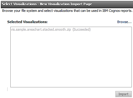
) and browse to your downloaded visualization zip file.
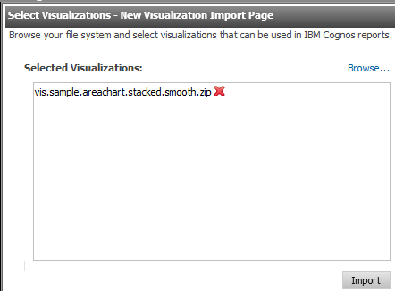
New Visualization
Click Import.
Selected Visualizations
Note: There is no need to restart services after the visualization(s) are imported.

Using Visualizations in Active Report

Now that the visualization is installed, let’s make our way over to Report Studio and create a Blank Active Report.
Active Report
You’ll notice there is a new Toolbox item called Visualization. We can drag and drop that into our page and find that we can now browse our gallery of visualizations from within Report studio. At this point we are back into known territory and can utilize Report Studio to populate data and format as we see fit. As with all IBM Cognos charts (both legacy and current), each type of visualization may have their own unique set of formatting options and functionalities.
Stacked Visualization
Below are screenshots of some Active Reports were created using GOSALES (query) data.
Active Report Example
Active Report Example 2

Active Report Example 3
 Comparing IBM Cognos RAVE vs. Tableau, Tibco and Qlikview
Adoption of data visualizations has grown significantly in recent years, as evidenced by an upswing for visually dominant tools in the Gartner Magic Quadrant Survey for Business Intelligence and Analytics Platforms. From 2011 to 2014, tools such as Tableau, Tibco Spotfire, and Qlikview have moved from in or near the challengers quadrant to the leaders quadrant, alongside more traditional BI tools, like IBM Cognos, Microsoft, and SAS. Additionally, the TDWI Best Practices report, Visual Reporting and Analysis: Seeing is Knowing, has indicated that this growth has not yet peaked. According to their research, “data visualization is in the middle of a remarkable growth phase” and contributes significantly to increased insight and productivity.
While historically IBM Cognos has not been lauded for its aesthetics, times have changed and so has IBM Cognos BI for the better. Advances in Cognos visual capabilities with Cognos 10+ have reduced the need to leverage additional tools to present data in its most visually appealing format. With the advent of RAVE (Rapidly Adaptive Visualization Engine) visualizations, particularly when used with Active Reports, Cognos users can experience interactive visualizations every bit as powerful and beautiful as those found in those other visual analytics tools. Combine that with your enterprise data via native mobile delivery (tablet) and you’ve got all you need to present your data in a stunning and easy to interpret format.
ActiveReportExample


A picture is worth a thousand words

Let’s compare some of the visualizations side by side so you can see for yourself the appeal of RAVE visualizations.  (Chart Descriptions courtesy of AnalyticsZone.com). The software versions used in this comparison were IBM Cognos 10.2.1, Tableau 8.2 (Trial Version),  Qlikview 11 (Trial Version), and Spotfire Cloud.
Editor’s Note: Since initial publication of this article, it has been brought to our attention that additional functionality and visualizations are available in the full Qlikview tool that may not be represented in this comparison. Namely, Gantt Charts and Box Plots are native chart types available in Qlikview.

Bar Chart

Bar charts use horizontal data markers to compare individual values. You can use bar charts to compare discrete data or show trends over time. Use clustered bar charts to compare values across multiple categories.
Bar

Line Chart

Line charts plot data at regular points connected by lines. You can use line charts to show trends over time and compare many data series.
Line

Pie Chart

Pie charts use segments of a circle to show the relationship of parts to the whole. You can use pie charts to highlight proportions.
Pie

Stacked Area Chart

Area charts are like line charts, but the areas below the lines are filled with colors or patterns. Stacked area charts are used to show the relationship of parts to the whole. You can use area charts to emphasize the magnitude of change over time.
AreaLine

Scatter Plot

Scatter charts use data points to plot two measures anywhere along a scale, not only at regular tick marks. You can use scatter charts to explore correlations between different measures.
Scatter

Treemap

Treemaps show relationships among large numbers of components using size and color in a set of nested rectangles. You can use treemaps to identify patterns and exceptions.
Treemap

Gantt Chart

Gantt charts are bar charts that illustrate a schedule or timeline by showing activities displayed against a date or time series.
Gantt

Packed Bubble

A packed bubble chart contains bubbles that are tightly packed rather than spread over a grid. You can use packed bubble charts to display a large amount of data in a small space.
PackedBubble

Box Plot

Box plots show the statistical summary of a distribution of numbers, such as median values, upper and lower quartiles and outliers.
BoxPlot

Bonus

You’ve seen in some of the above comparisons that occasionally tools lack visualizations that others have. What if you happen to need a visualization that isn’t available? With IBM Cognos BI and RAVE Visualizations you can create it using the RAVE design language and the freely available RAVE customization tool.
Custom
Visit Analytics Zone and explore the robust inventory of existing visualizations. Simply download and import the visual you want to leverage and you will be on your way to creating captivating reports and dashboards.